
Beautiful tables with gt and gtExtras
Tom Mock
![]()
A grammar of graphics1
Easy enough to rapidly prototype graphics at the “speed of thought”

Powerful enough for final “publication”

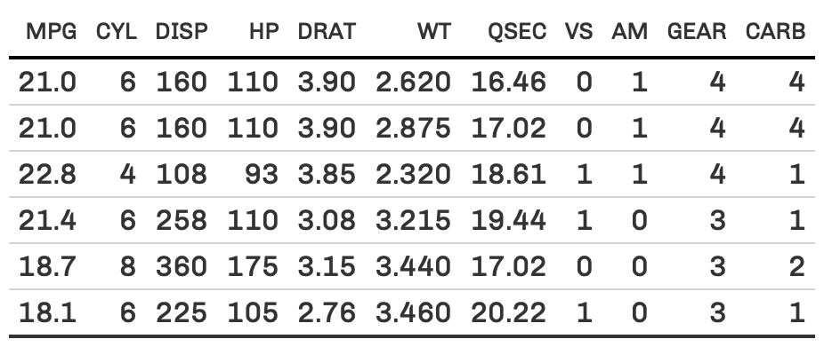
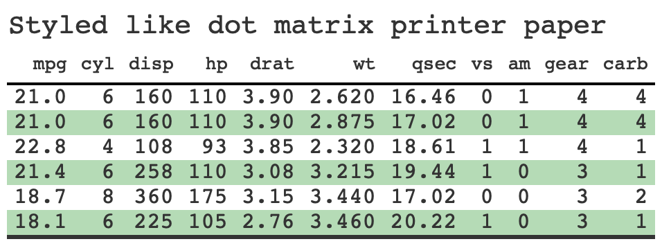
Tables with R
Construct a wide variety of useful tables with a cohesive set of table parts. These include the table header, the stub, the column labels and spanner column labels, the table body and the table footer.


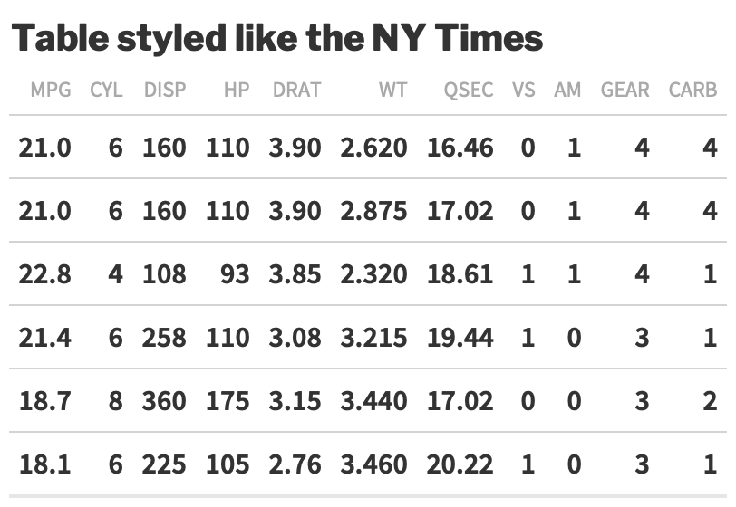
Easy enough to rapidly prototype

Powerful enough for final “publication”

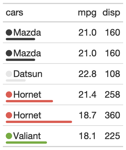
What about merging graphs AND tables?
🌶️ Hot take - Horizontal bar charts and simple charts with facets are already tables.

| body_mass | plot | |
|---|---|---|
| Adelie | ||
| male | 4,043.49 | |
| female | 3,368.84 | |
| Chinstrap | ||
| male | 3,938.97 | |
| female | 3,527.21 | |
| Gentoo | ||
| male | 5,484.84 | |
| female | 4,679.74 | |
Hot take, continued


![]()
Themes
Sparklines

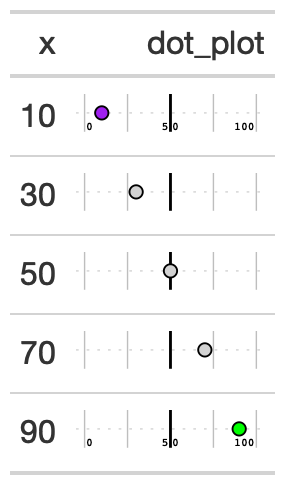
Dot + Bar
Point
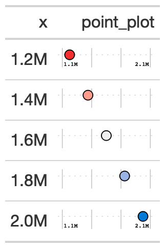
Percentile
Confidence interval
# gtExtras can calculate basic conf int
# using confint() function
ci_table <- generate_df(
  n = 50, n_grps = 3,
  mean = c(10, 15, 20), sd = c(10, 10, 10),
  with_seed = 37
) %>%
  dplyr::group_by(grp) %>%
  dplyr::summarise(
    n = dplyr::n(),
    avg = mean(values),
    sd = sd(values),
    list_data = list(values)
  ) %>%
  gt::gt() %>%
  gt_plt_conf_int(list_data, ci = 0.9)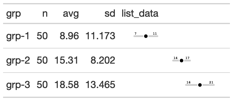
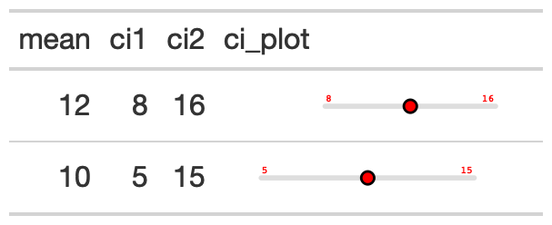
Confidence interval, user defined
# You can also provide your own values
# based on your own algorithm/calculations
pre_calc_ci_tab <- dplyr::tibble(
  mean = c(12, 10), ci1 = c(8, 5), ci2 = c(16, 15),
  ci_plot = c(12, 10)
) %>%
  gt::gt() %>%
  gt_plt_conf_int(
    column = ci_plot,
    ci_columns = c(ci1, ci2),
    palette = c("red", "lightgrey", "black", "red")
    )
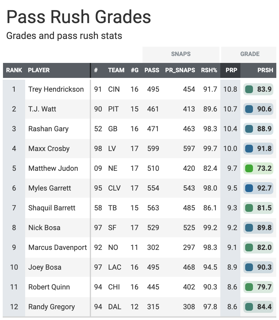
gt + Plots

gt + Plots

You can write your own gt “extra” functions!
![]()